
输入“一本书和一台笔记本电脑”,模型画出了一台电脑,却忘了书。再试一次,书出现了,电脑又不见了。既然模型偶尔能画对,能不能多花一些生成时的计算,让它更经常画对?
最直接的办法是多生成几张,最后挑一张。更主动的办法是:图像还没画完,就判断哪些方向更有希望,把后续计算放在那里。
但中途的判断可能不准;很多条生成路径,也可能在反复筛选后变成同一个祖先的后代。我们既希望计算用得更有效,也希望最后的概率分布没有被错误判断带偏。
这篇博客沿着一条线展开:URGE 用路径信息校正引导;独立拒绝避开共同祖先;Stein Guidance 则让引导和校正都只依赖函数值。这里的“无导数”指不必对价值函数求导,基础去噪模型仍照常运行。[1][2]
1. 多算一点,究竟想得到什么?
把扩散模型想成一个随机的绘画过程:从噪声出发,逐步去噪,最后生成图像。本文沿生成方向记时间,\(0\) 是开始,\(T\) 是完成。训练好的模型对应基础分布 \(p_{\mathrm{base}}\)。
给成品一个分数 \(r(x)\),再把它变成正的偏好权重 \(\phi(x)=e^{\beta r(x)}\),就得到我们希望采样的分布:
\[\pi(x)=\frac{p_{\mathrm{base}}(x)\phi(x)} {\mathbb E_{p_{\mathrm{base}}}[\phi(X)]}.\]它保留模型原本的生成偏好,同时提高高分结果的相对概率。\(\beta\) 控制偏好强度。[1, §2.1]
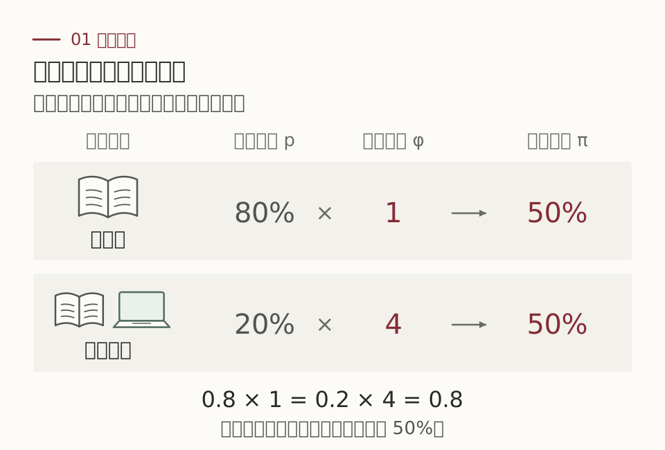
这个采样目标与“找到最高分的一张图”有关,但并不相同。例如,独立生成多张后取最高分,一般不会得到上面的 \(\pi\)。下面的“校正正确”,都针对这个明确的分布目标。
增加计算也有三种不同方式:更多去噪步 \(n\),更多生成路径 \(N\),或者每一步更多候选 \(K\)。它们分别增加数值深度、统计宽度和局部查询量,不能混成一个“采样次数”。[2, §1]
2. 想知道下一步怎么走,先问它的未来
半成品还很模糊,直接问“现在像不像一本书”,未必能判断最后画得好不好。更合理的问题是:从这个状态继续生成,最终偏好权重的平均值是多少?
\[H_t^\star(x)=\mathbb E[\phi(X_T)\mid X_t=x].\]这个价值函数把未来的可能性都考虑进来。如果它精确已知,下一步就可以按照“基础转移概率 × 下一步的价值”抽样。在连续时间里,相应的引导漂移是 \(\sigma\sigma^\top\nabla\log H_t^\star\),也就是 Doob 变换。[1, §1][2, §3]
困难在于:\(H^\star\) 本身就包含一个高维积分。实践中通常只能得到近似价值 \(H\),例如先预测最终图像,再对预测结果打分。
因此,需要把两件事分开:近似价值负责指路,校正机制负责处理指错路造成的概率偏差。判断越好,校正通常越容易,但正确性不能建立在每次判断都准确之上。
3. URGE:把整条生成路径的账算清楚
引导改变了模型的走法。同一个终点可以从许多不同路径到达,因此很难直接计算引导后的终点密度。URGE 的切入点是:保留实际走过的路径,对这条路径计算概率比。[1, §2.3]
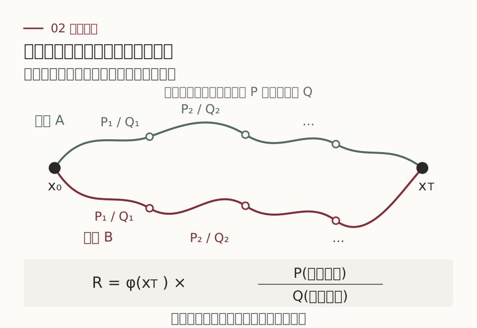
离散时间里,设基础转移密度是 \(P_k\),实际提议密度是 \(Q_k\),二者使用相同的初始分布,并满足概率比所需的支持条件。对实际生成的路径记录
\[R=\phi(X_n)\prod_{k=0}^{n-1} \frac{P_k(X_k,X_{k+1})}{Q_k(X_k,X_{k+1})}.\]被引导抽得过于频繁的路径,权重要压下来;被抽得太少的路径,权重要补上去。最终偏好告诉我们想要什么,概率比补偿实际怎样抽样。
连续时间里对应 Girsanov 换测度。URGE 利用模拟时的漂移与随机增量计算路径权重,并在生成过程中重加权、重采样。它本身也是 SMC,路径权重与粒子权重的关系可以展开下面的说明。[1, §2.3]
URGE 与粒子 SMC:对终点取条件平均,省下导数又多了什么方差?
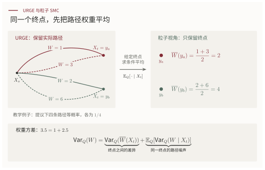
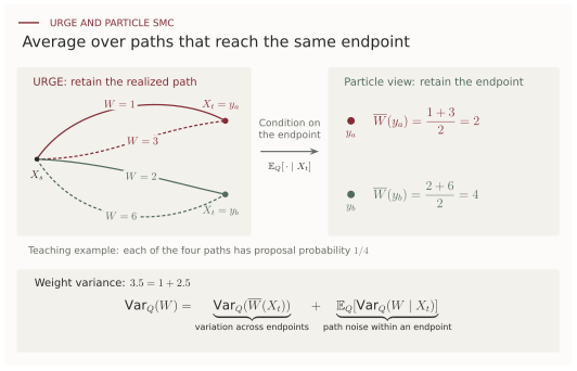
一条路径记一笔账,还是同一终点先合并账目? 两种方法都传播、加权、重采样。URGE 的权重依赖实际走过的路径;粒子视角把抵达同一终点的路径按条件概率平均,只保留当前状态需要的权重。这里讨论的粒子校正具体指 FK Corrector/AFDPS。
在同一个提议律 \(Q\) 下,记一段路径的权重为 \(W\)。给定终点后,把未观察到的路径平均掉,得到
\[\overline W(x)=\mathbb E_Q[W\mid X_t=x].\]直觉上,终点都是同一个 \(x\),最终统计就不必再区分它是绕远路还是走近路到达的。对任意合适的终点函数 \(f\),条件期望的塔式法则给出
\[\mathbb E_Q[Wf(X_t)] =\mathbb E_Q[\overline W(X_t)f(X_t)].\]所以,先按路径加权再只看终点,与先对路径权重取条件平均再给终点加权,得到相同的加权边际分布。归一化常数也相同,因为可以取 \(f=1\)。
对于 URGE 的短路径增量,论文在相应正则性与边际匹配条件下进一步得到
\[\lim_{h\downarrow0} \frac{\mathbb E_Q[W_{t-h,t}\mid X_t=x]-1}{h} =\lambda_{\mathrm{particle}}(x,t),\]右边就是 FK Corrector/AFDPS 的粒子校正势。有限区间上有精确的条件平均恒等式;与论文中粒子校正势的对应,则要取短时间极限。 这不表示两个有限粒子实现每次重采样会选中同样的粒子。[1, Theorem 3.3]
好处:用 Itô 公式,把导数账改写成路径上可直接记录的增量。 设 \(\ell_t\) 是中间偏好权重的对数,终点满足 \(\ell_T=\log\phi\);引导后的提议写成 \(dX=(b+\sigma u)\,dt+\sigma\,dB^Q\)。URGE 的增量权重可写为
\[\log W_{s,t} =\ell_t(X_t)-\ell_s(X_s) -\int_s^t u_\tau^\top dB_\tau^Q -\frac12\int_s^t\|u_\tau\|^2d\tau.\]这里用的是两端的函数值、实际漂移变化与已经模拟出的噪声。为什么它能替代包含导数的表达?Itô 公式把同一个函数增量写成
\[d\ell_t(X_t) =\left[\partial_t\ell_t+(b+\sigma u)\cdot\nabla\ell_t +\tfrac12\operatorname{tr}(\sigma\sigma^\top\nabla^2\ell_t)\right]dt +(\sigma^\top\nabla\ell_t)^\top dB_t^Q.\]从右边看,有时间导数、梯度和 Hessian;沿已模拟的路径计算左边,只需函数值的差。结合 Girsanov 路径比,就能避免为校正额外求这些导数或边际 score。若构造 guidance 本身仍采用 \(u=\sigma^\top\nabla G\),这部分已有的引导梯度仍要计算。
代价:同一终点下,走过哪条路仍会让权重波动。 若 \(W\) 二阶可积,全方差公式给出
\[\operatorname{Var}_Q(W) =\operatorname{Var}_Q(\overline W(X_t)) +\mathbb E_Q[\operatorname{Var}_Q(W\mid X_t)] \ge\operatorname{Var}_Q(\overline W(X_t)).\]条件平均是一次 Rao–Blackwell 化:它消掉了终点相同、路径不同所带来的权重噪声。URGE 直接使用实际路径权重,省去了求这个条件平均或显式导数的成本,却保留了这部分额外方差;只要同一终点下权重确有波动,不等式就是严格的。
Itô 改写本身是恒等式,不会增加方差;增加的是相对于精确条件平均权重而言,保留路径随机性的代价。 上面的比较针对同一提议下的原始权重,实际算法的最终误差还受离散化、导数估计、重采样和计算预算影响。
4. 多条路径,可能已经变成一家人
SMC 不断复制高权重粒子,淘汰低权重粒子。复制的并不只是一个分数,而是粒子当前的状态,以及通向这个状态的整段历史。所以,屏幕上还剩多少粒子,与它们保留了多少份独立的早期探索,是两件事。
想象四个人各自解题,每隔一会儿,都按评分挑一份草稿接着写。几轮以后,桌上仍有四份答卷,却可能都源自同一份早期草稿。后面写得再不一样,最初的关键选择也已经被一起继承了。
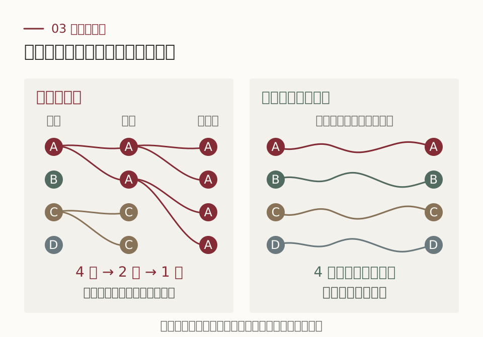
沿左图看:第一轮只保留 A、C 的后代,B、D 的早期探索消失;第二轮只留下 A 家族。此时的四个粒子可以位于不同位置,却都受同一段早期随机历史影响。右图则让四次完整生成各用各的随机数,保留四份独立的探索机会。
一个简化例子能说明这为什么影响统计精度。假设最终结果可写成 \(X_T^{(i)}=A+\varepsilon_i\):\(A\) 是大家继承的随机前缀,后续噪声 \(\varepsilon_i\) 相互独立、同分布,并且独立于 \(A\)。平均 \(N\) 个后代后,
\[\operatorname{Var}\!\left(\frac1N\sum_{i=1}^N X_T^{(i)}\right) =\operatorname{Var}(A)+\frac{\operatorname{Var}(\varepsilon_1)}N.\]后半程的独立噪声可以靠平均降低,大家共同继承的早期误差却不会被这次平均消掉。 这是一个解释相关性的教学模型,不是所有扩散过程都具有这种加法形式。
ESS 只看当前权重是否均匀。重采样后权重通常重新设为相等,因此即使四个粒子全是 A 家族,也可以有 \(\mathrm{ESS}=N\)。它没有记录家谱,不能据此认定粒子独立。增加去噪步若也增加重采样次数,就可能带来更多祖先合并的机会。[2, §1、附录 E]
一个严格的反例:每步重采样,误差可能随深度累积
文献 [2] 构造了一个布朗运动例子:终点目标固定,局部 Bellman 误差为 \(O(1/n)\);若每个数值步都做完整的多项分布重采样,一个最终粒子的分布满足
\[\left\|\nu_{n,N}^{\mathrm{SMC}}-\pi\right\|_{\mathrm{TV}} \asymp\frac nN,\qquad 2\le n\le N.\]这里的总变差距离衡量两个分布对同一事件给出的概率最多能差多少。这个结果针对论文构造的模型和每步完整重采样,不能外推为所有 SMC 的下界,也不排除稀疏或自适应重采样的价值。[2, Theorem 1]
5. 不复制别人的路径,为什么仍要校正?
拒绝这一步,保留自己的草稿
一个自然的替代是逐步拒绝采样(sequential rejection sampling):从当前状态试走一步,按候选价值决定接受还是拒绝。拒绝后保留自己的前缀,只重新尝试这一步,而不是复制另一个人的历史。
若有已知有效上界 \(0<H_{k+1}(y)\le M_k(x)\),就从基础转移 \(P_k(x,\cdot)\) 抽取候选 \(Y\),以 \(H_{k+1}(Y)/M_k(x)\) 的概率接受,重复到接受后再前进。独立重跑整套路径生成程序,各条路径就没有跨路径的共同祖先。这是下图右侧的机制。
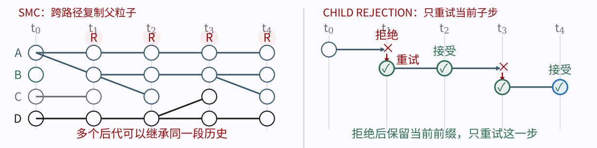
它也不同于后面“整条路径生成完以后,再做外层 MH 校正”:这里拒绝的是一个子步;后者接受或保留的是一条完整提议。
没有共同祖先,不等于中途不会指错路
SMC 的一个好处是保留沿途的权重账本。例如,固定起点,并令终点价值 \(H_n=\phi\),在基础转移下使用增量权重 \(H_{k+1}(X_{k+1})/H_k(X_k)\),就有
\[\frac{H_1(X_1)}{H_0(X_0)} \frac{H_2(X_2)}{H_1(X_1)}\cdots \frac{\phi(X_n)}{H_{n-1}(X_{n-1})} =\frac{\phi(X_n)}{H_0(X_0)}.\]中间判断像暂记的账:前一步记上,后一步扣回。因此,中间价值不必等于真实未来价值,正确的未归一化目标仍由终点偏好决定。这里说的是权重构造的恒等式,不是有限粒子的 SMC 已经精确。[2, 附录 E.2]
只做局部拒绝则不同。每一步都把候选价值重新归一化成概率,分母是“从当前状态出发,下一步价值的真实平均”,不一定等于当前的近似预测。相邻的价值项仍能相消,但预测与实际平均不一致留下的比值,通常消不掉。[2, §3、式 (10)–(11)]
用一个两步教学例子就能看清。基础模型等概率选择路线 A、B;选定后各自到达不同终点,两个终点的真实偏好都为 1。因此目标应当各占一半。可是中途的预测把 A 评为 9、B 评为 1:
| 两条互不相通的路线 | 目标概率 | 中途预测 | 局部拒绝后的概率 |
|---|---|---|---|
| A | 50% | 9 | 90% |
| B | 50% | 1 | 10% |
到终点时,两边的奖励都算对了,却都等于 1,后一步没有任何筛选差别。于是,前面多给 A 的机会,不会因为终点打分正确而自动退回来。
校正需要把 A 的相对权重乘以 \(1/9\),B 乘以 \(1\);两边加权质量都是 \(0.1\),重新归一化才恢复各 \(50\%\)。也可以在最后以 \(1/9\) 的概率接受 A、总是接受 B:补回概率,不需要复制别人的前缀。这组数字是教学例子,不是论文实验。
把这笔账写成公式:局部精确,为什么全局仍可能有偏?
按本文记号,令
\[G_k(x)=(P_kH_{k+1})(x),\qquad Q_k^H(x,dy)=\frac{P_k(x,dy)H_{k+1}(y)}{G_k(x)}.\]有效包络下的局部拒绝能精确模拟 \(Q_k^H\)。但相对于最终目标 \(\Pi_n\propto\phi(X_n)P_n\),整条路径仍有权重
\[R_H=\phi(X_n)\frac{dP_n}{dQ^H}(X_{0:n}) =H_0(x_0)\prod_{k=0}^{n-1}\frac{G_k(X_k)}{H_k(X_k)}.\]精确 Doob 价值满足 \(G_k=H_k\),这时权重为常数,局部采样就够了。近似价值一般留下依赖路径的乘积;如果这个乘积恰好为常数,也不需要校正。否则它就是漏掉的完整路径校正。[2, §3、附录 C.3]
对于上面的两步例子,\(G_0=5\),而 \(G_1(A)=G_1(B)=1\),因此精确路径权重分别为 \(5/9\) 和 \(5\)。省略两者共同的因子 5,就是正文中的 \(1/9\) 与 \(1\)。
困难是 \(G_k\) 本身是积分,通常不能精确计算。有限候选池的作用不仅是帮我们选下一步,还要提供可计算的校正信息。若起点随机,初始分布的因子也必须纳入分析,不能直接套用固定起点下的常数结论。[2, Proposition 22]
显式 guidance 的另一笔成本:为什么校正会碰到二阶导数?
先看指路。把漂移改为 \(b+a\nabla\log H\),其中 \(a=\sigma\sigma^\top\),只需知道价值在当前位置往哪个方向上升,因此要算一阶导数。可是 \(H\) 是近似的;走完整条路径以后,我们还要知道:这些中途判断累计把抽样概率改偏了多少,最后该以多大权重保留这条路径?
上一段的离散校正已经给出了线索:每一步留下 \(G_k/H_k\),其中 \(G_k=P_kH_{k+1}\)。分子是“按基础动力学走一步后,下一时刻价值的真实平均”,分母是“当前位置对未来的预测”。精确价值让两者一致;近似价值留下的差,就是要沿途累计的 Bellman 缺陷。
为什么算这个平均会遇到二阶导数? 随机步既可能向左,也可能向右。向两边的一阶变化在平均时抵消,但两边共同向上或向下弯的部分会留下。暂时忽略时间与漂移,一维 Taylor 展开是
\[H(x+\sqrt h Z) =H(x)+\sqrt h\,H'(x)Z+\frac h2 H''(x)Z^2+\cdots, \qquad Z\sim N(0,1).\]由于 \(\mathbb EZ=0\)、\(\mathbb EZ^2=1\),在相应光滑性与可积性条件下,
\[\mathbb E[H(x+\sqrt h Z)]-H(x) =\frac h2 H''(x)+o(h).\]例如 \(H_+(x)=e^{cx^2}\) 与 \(H_-(x)=e^{-cx^2}\),其中 \(c>0\)。在 \(x=0\),它们的价值都为 1,梯度都为 0,因而给出同样的瞬时引导;但前者是谷底,后者是坡顶。随机走一小步,平均价值分别变为 \(1+ch+O(h^2)\) 与 \(1-ch+O(h^2)\)。相同的价值和梯度,需要方向相反的局部概率补偿;缺失的信息就在曲率里。
把时间变化、基础漂移和多维噪声一起放回去,每单位时间的相对缺陷就是
\[\mathcal E_t(x) =\frac{\partial_tH_t+b_t\cdot\nabla H_t +\tfrac12\operatorname{tr}(a_t\nabla^2H_t)}{H_t}(x).\]三项分别记录价值随时间的变化、基础漂移造成的变化,以及噪声遇到曲率时造成的平均变化。最后一项是 Hessian 与噪声协方差的收缩;未必需要显式存储整个 Hessian,但仍需二阶空间导数信息。
这与最后的接受或拒绝有什么关系? 在固定起点、\(H_T=\phi\)、正且足够光滑的 \(H\) 以及合法换测度等条件下,对漂移为 \(b+a\nabla\log H\) 的连续时间提议,完整路径的未归一化校正权重满足
\[R_H=H_0(x_0)\exp\!\left(\int_0^T\mathcal E_t(X_t)\,dt\right).\]终点偏好已经通过 \(H_T=\phi\) 进入这个恒等式。剩下的指数项累积整条路上的概率补偿,最终进入新旧路径的 MH 权重比;若另有有效权重上界,也可以据此做完整路径拒绝采样。接受概率的公式很简单,困难在于把其中的路径权重算出来。沿残差这条路线,梯度负责 guidance,时间导数与二阶空间导数参与 correction。 离散时对应上一段的 \(\log(G_k/H_k)\) 累积。[2, §4、式 (11)]
为什么 URGE 又能避开显式 Hessian?
上式把路径概率比整理成了价值函数的残差。URGE 保留实际漂移与噪声增量,直接用 Girsanov 路径比计算校正,因此可以绕开显式时间导数和 Hessian。若漂移本身采用 \(\nabla\log H\),构造提议仍要计算价值梯度。高阶导数是直接计算残差的成本,并不是所有校正方法都不可避免的成本。 [1, §2.2–2.4]
连续时间的恒等式也不意味着任意离散实现自动精确。实际算法必须使用与其离散提议匹配的校正权重。
现在要设计的是一对配套机制:用函数值把路径引向好区域,同时留下可以用函数值算清的概率账本。 下一节从两个对称候选开始,看看这两件事怎样共用同一批查询。
6. 两个对称候选,为什么产生对数梯度?
对称差分给出价值的方向导数,选择概率的归一化再除以当前价值,因此出现的是 \(\nabla H/H=\nabla\log H\)。
具体地,记基础漂移后的位置为 \(\mu=x+hb(x)\),取一个高斯扰动 \(\delta=\sqrt h\,\sigma Z\),其中 \(Z\sim N(0,I)\)。构造两个对称候选,并查询它们的价值:
\[Y^\pm=\mu\pm\delta,\qquad H^\pm=H(Y^\pm).\]按概率 \(p_\pm=H^\pm/(H^++H^-)\) 选择一个候选。给定当前状态与扰动,平均位移恰好是
\[\mathbb E[Y^J-\mu\mid x,Z] =\delta\frac{H^+-H^-}{H^++H^-}.\]对两侧函数值作一阶展开:相减时,常数项相消,留下 \(2\delta^\top\nabla H(\mu)\);相加时,主项是 \(2H(\mu)\)。所以小扰动下,
\[\frac{H^+-H^-}{H^++H^-} \approx\frac{\delta^\top\nabla H(\mu)}{H(\mu)} =\delta^\top\nabla\log H(\mu).\]代回平均位移,便得到主项 \(\delta\delta^\top\nabla\log H(\mu)\)。再对随机方向取平均,利用 \(\mathbb E[\delta\delta^\top\mid x]=h\sigma\sigma^\top\),得到
\[\mathbb E[Y^J\mid x] =\mu+h\sigma\sigma^\top\nabla\log H(\mu)+o(h).\]这就是按噪声协方差调整后的对数梯度引导。执行时只查询两次函数值,再按比例选一个候选;梯度来自对平均位移的分析,不需要实际计算。 上述小步长结论要求 \(H\) 光滑、为正且余项可积,描述的是一阶平均漂移,有限步的转移分布仍需校正。[2, §3.1.1、式 (5)、附录 B.2.1]
7. Stein 恒等式:把两点推广到 K 个并行候选
两个点揭示了方向信息。能否同时查询 \(K\) 个方向,并仍然只用函数值?高斯 Stein 恒等式给出连接:
\[\mathbb E[Zf(Z)]=\mathbb E[\nabla f(Z)],\qquad Z\sim N(0,I).\]左边只用函数值,右边是梯度的平均。直觉是:哪个方向更常得到高价值,“随机方向 × 价值”的平均就偏向哪里。对 \(Y=\mu+\sqrt h\,\sigma Z\),它给出
\[\mathbb E[ZH(Y)]=\sqrt h\,\sigma^\top\mathbb E[\nabla H(Y)].\]这在相应高斯分部积分条件下成立。[2, §3.1.2、Proposition 6]
保留对称性:让整组方向加起来为零
两点方法满足 \(Z_1+Z_2=0\)。推广到 \(K\ge2\),先抽取独立标准高斯 \(G_i\),减去平均,再恢复每个方向的方差:
\[\bar G=\frac1K\sum_iG_i,\qquad Z_i=\sqrt{\frac K{K-1}}(G_i-\bar G),\qquad \sum_iZ_i=0.\]每个 \(Z_i\) 单独看仍是标准高斯,池内则相互依赖。随后构造候选,同时查询全部价值,再按价值比例随机选一个:
\[Y_i=\mu+\sqrt h\,\sigma Z_i,\qquad H_i=H(Y_i),\qquad \Pr(J=i\mid Y_{1:K})=\frac{H_i}{\sum_jH_j}.\]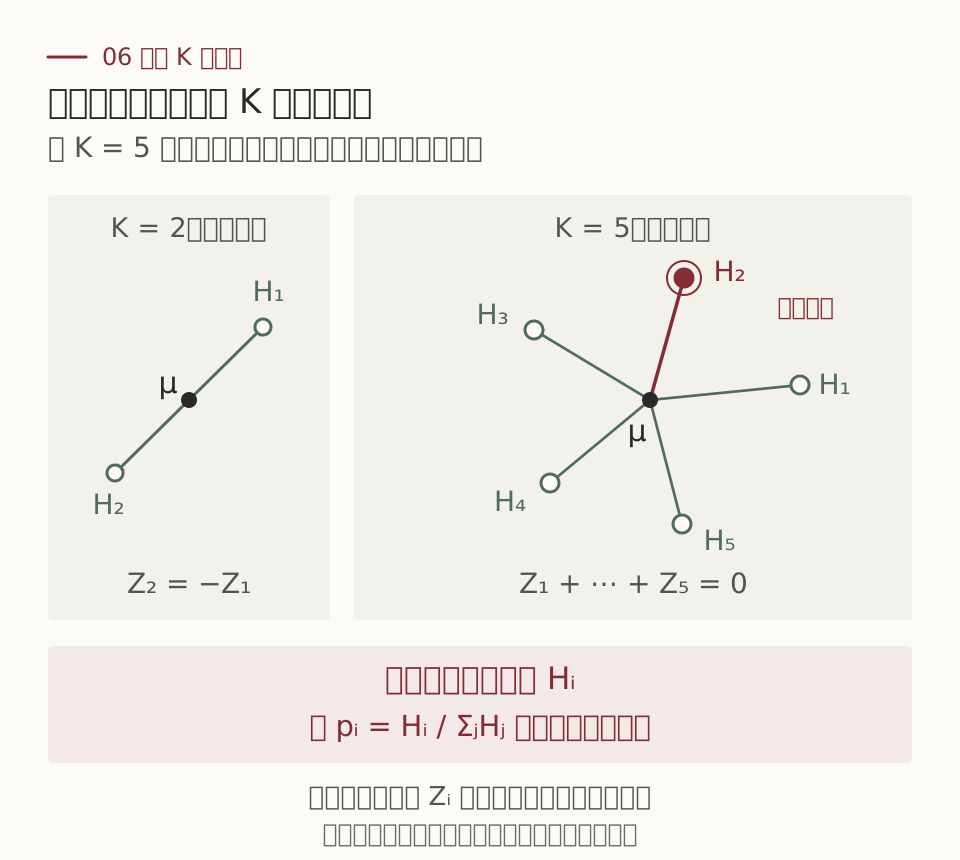
给定候选池 \(U\),选择产生的平均位移恰好为
\[\mathbb E[Y_J-\mu\mid U] =\sqrt h\,\sigma\frac{\sum_iZ_iH_i}{\sum_iH_i}.\]这就是用有限次查询,替换理想价值倾斜中的期望。\(K=2\) 时,\(Z_1=(G_1-G_2)/\sqrt2=-Z_2\),恰好回到刚才的有限差分。构造也支持奇数 \(K\),不必成对分组。[2, 式 (7)–(8)]
为什么中心化让方差多改善一阶 h?
候选扰动是 \(\sqrt h\) 量级。中心化把泰勒展开中的一阶随机项精确消掉,留下 \(h\) 量级的二阶波动;波动平方以后,方差就从 \(h\) 量级变成 \(h^2\) 量级。 下面把这个计算写出来。[2, Remark 2]
固定当前状态,将 \(\mu,\sigma\) 视为已知。我们关心的是候选价值平均 \(S=K^{-1}\sum_iH(\mu+\sqrt h\,\sigma Z_i)\) 的波动,记它的真实均值为 \(G_h=\mathbb ES\),并简写
\[g=\sigma^\top\nabla H(\mu),\qquad A=\sigma^\top\nabla^2H(\mu)\sigma,\qquad \bar Z=\frac1K\sum_iZ_i.\]对每个候选的价值作二阶泰勒展开,再取平均并减去期望,得到
\[\begin{aligned} S-G_h &=\sqrt h\,g^\top\bar Z\\ &\quad+\frac h{2K}\sum_{i=1}^K \left(Z_i^\top AZ_i-\operatorname{tr}A\right)+r_h. \end{aligned}\]第一行是梯度带来的一阶噪声,第二行是曲率带来的二阶噪声。以下渐近式固定 \(K\)、令 \(h\to0\);当 \(H\) 二阶连续可微且 Hessian 有界时,余项 \(r_h\) 的均方根是 \(o(h)\)。
独立候选:一阶项只在期望中为零。 若 \(Z_i\) 相互独立,虽然 \(\mathbb E\bar Z=0\),单次抽样的 \(\bar Z\) 仍然随机,而且 \(\operatorname{Cov}(\bar Z)=I/K\)。因此,一阶项通常主导方差:
\[\operatorname{Var}(S_{\mathrm{iid}}) =\frac{h\|g\|^2+o(h)}{K}.\]中心化候选:一阶项在每次抽样时都为零。 上面的构造保证 \(\sum_iZ_i=0\),所以 \(\sqrt h\,g^\top\bar Z\) 整项消失。剩下的主导随机项前面是 \(h\),不再是 \(\sqrt h\)。将二次项的方差算出,便得到
\[\operatorname{Var}(S_{\mathrm{centered}}) =\frac{h^2}{2(K-1)}\|A\|_F^2+o(h^2).\]这里 \(\|A\|_F^2\) 是矩阵元素的平方和。多出来的一阶 \(h\),来自随机波动由 \(\sqrt h\) 降到 \(h\),再对它平方;不是靠增加候选数量得到的。
每个中心化方向仍是标准高斯,因此两种构造都满足 \(\mathbb ES=G_h\),估计的是同一个归一化常数。若 \(G_h\) 有统一正下界,除以 \(G_h^2\) 不改变上述方差的阶,于是归一化平均值 \(S/G_h\) 的方差从 \(O(h/K)\) 改善为 \(O(h^2/(K-1))\)。这说的是随机误差;\(G_h\) 与 \(H(\mu)\) 之间的平滑差异仍可为 \(O(h)\)。若 \(g=0\),独立候选的一阶项本来也为零。
把系数算完整:分母为什么是 K−1?
中心化方向彼此相关:
\[\operatorname{Cov}(Z_i,Z_j)=-\frac{I}{K-1}, \qquad i\ne j.\]记 \(q_i=Z_i^\top AZ_i\)。高斯四阶矩公式给出
\[\operatorname{Var}(q_i)=2\|A\|_F^2,\qquad \operatorname{Cov}(q_i,q_j) =\frac{2\|A\|_F^2}{(K-1)^2}\quad(i\ne j).\]因此,计算平均值的方差时,要把对角项和交叉项都加起来:
\[\begin{aligned} \operatorname{Var}\!\left(\frac1K\sum_iq_i\right) &=\frac{2\|A\|_F^2}{K^2} \left(K+\frac{K(K-1)}{(K-1)^2}\right)\\ &=\frac{2\|A\|_F^2}{K-1}. \end{aligned}\]再乘泰勒二次项前系数的平方 \(h^2/4\),就得到 \(h^2\|A\|_F^2/[2(K-1)]\)。方向之间的负相关消掉了一阶噪声,但二次项的协方差为正,所以这里要使用它们的实际联合分布。[2, 附录 B.3]
不只看渐近主项,也有真正的上界。 令 \(F(z)=H(\mu+\sqrt h\,\sigma z)\)。当 \(F\) 及其前两阶导数在标准高斯分布下平方可积,且 \(G_h>0\) 时,文献 [2, Theorem 8] 给出对每个 \(K\ge2\) 成立的界:
\[\operatorname{Var}\!\left(\frac S{G_h}\right) \le \frac{h^2}{2(K-1)G_h^2} \mathbb E\left\| \sigma^\top\nabla^2H(\mu+\sqrt h\,\sigma Z)\sigma \right\|_F^2.\]相对曲率项有统一上界时,就得到统一的 \(O(h^2/(K-1))\) 保证。这里出现 Hessian 是为了分析误差;实际构造候选、计算 \(S\) 和路径校正时,仍然只使用函数值。
函数值估计无偏,为什么最后的引导仍可能有偏?
令 \(G=\mathbb E[H(Y)]\)。Stein 恒等式保证
\[\widehat v=\frac1{K\sqrt h}\sum_iZ_iH(Y_i),\qquad \mathbb E\widehat v=\sigma^\top\mathbb E\nabla H(Y),\qquad \mathbb ES=G.\]但一般 \(\mathbb E[\widehat v/S]\ne\mathbb E[\widehat v]/\mathbb E[S]\)。分子和分母分别无偏,不代表比值无偏。因此,有限池近似和不精确价值造成的路径偏差,仍要用下一节的权重处理。[2, Proposition 6、Theorem 11]
8. 生成完以后,再校正整条路径
第 5 节留下一个问题:理想局部归一化常数 \(G_k=P_kH_{k+1}\) 不好算。有限候选池提供了一个出口:不用精确求这个积分,保留同一批查询的平均值,也能构造正确的扩展空间权重。[2, §3.2、Theorem 12]
\[R=\phi(X_n)\prod_{k=0}^{n-1} \frac{S_k}{H_{k+1}(X_{k+1})},\qquad S_k=\frac1K\sum_{i=1}^K H_{k+1}(Y_{k,i}).\]这个权重同时处理近似价值与有限候选选择留下的偏差,无需额外价值查询或导数。注意:它的正确性来自包含候选池与选择编号的扩展空间构造,不是把 \(G_k\) 随意替换成一个无偏估计就自动正确。
随后使用整条路径的独立提议 Metropolis–Hastings 更新。新旧路径权重分别为 \(R_{\mathrm{new}}\) 与 \(R_{\mathrm{old}}\),接受概率为
\[\alpha=\min\{1,R_{\mathrm{new}}/R_{\mathrm{old}}\}.\]接受就换成新路径;拒绝就保留旧路径和旧权重。比较的是经过概率补偿的路径权重,不能直接换成终点奖励。[2, Algorithm 2]
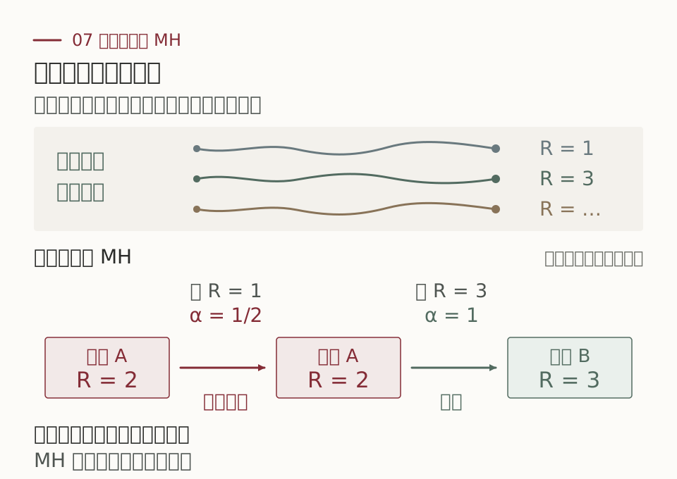
独立的是提议路径,一条 MH 链相邻的输出仍然相关。有限次更新也仍有初始化误差;若需要独立输出,应独立重复整套程序。已知有效全路径权重上界时,可另用完整路径拒绝采样获得独立的精确有限网格样本;这里主要讨论固定计算预算的外层 MH。[2, Algorithm 2、附录 G.2]
为什么这个权重有效?关键是一次精确消去
给定候选池,\(S=K^{-1}\sum_iH(Y_i)\),选择概率是 \(H(Y_i)/(KS)\)。因此
\[\mathbb E\!\left[\frac S{H(Y_J)}f(Y_J)\mid U\right] =\sum_i\frac{H(Y_i)}{KS}\frac S{H(Y_i)}f(Y_i) =\frac1K\sum_i f(Y_i).\]再对候选池取平均,每个候选都有正确的基础转移边际,右边便恢复基础转移。沿时间重复、最后乘上 \(\phi(X_n)\),得到
\[\mathbb E_{\widetilde Q}[RF(X_{0:n})] =\mathbb E_{P_n}[\phi(X_n)F(X_{0:n})].\]所以,这不是仅仅对“平均漂移”作校正,而是恢复正确的加权路径目标。相应 MH 的目标是不变分布,有限时间的接近程度还需要收敛分析。[2, Theorem 12]
9. 更多去噪步,能否不再强迫我们堆更多路径?
固定总时间 \(T\),步长 \(h=T/n\)。中心化候选每步的归一化方差是 \(O(h^2/(K-1))\),累积 \(n\) 步,对应的量级是
\[\frac{nh^2}{K-1}=\frac{Th}{K-1}.\]网格越细,这部分池噪声反而越小。但近似价值的 Bellman 误差是另一项,扩大候选池不能自动消除它。[2, §4]
在固定起点、\(H_n=\phi\)、统一正值上下界、二阶空间导数和噪声系数有界等条件下,论文证明:达到给定有限网格采样精度所需的完整提议数量,可以不随去噪深度增长。常数可以依赖维数与价值函数的界,并不声称维数无关。[2, Theorem 4]
这不意味着加深免费。\(m\) 次外层更新加一次初始化,共用 \(m+1\) 条完整提议,价值查询数仍是 \(Kn(m+1)\)。解决的是“每条路变长后,是否还被迫增加路的数量”,不是免去走更长路径的成本。
固定每条路径的查询预算,两个候选是否已经够好?
若单条提议预算 \(B=Kn\) 固定,则
\[\frac{Th}{K-1}=\frac{T^2}{B}\frac K{K-1}.\]对 \(K\ge2\),最后的因子介于 1 和 2 之间。仅从池噪声项看,两点已经获得相同的预算阶;更多候选可以增加并行度,但也减少预算内可走的步数,不能据此断言总误差一定更小。[2, §4]
这些结论针对离散模型的目标分布;它与连续时间扩散目标之间的数值误差需要单独分析。数值误差、价值近似误差和有限计算下的采样误差,应当分开记账。
10. 实验:先看 URGE,再看 Stein
URGE:先在“知道正确答案”的分布上检验
URGE 使用 30 维、40 个分量的高斯混合模型。加入二次奖励后,目标仍有解析表达,因而能直接检查分布是否采对。下表节选原论文 Table 2;两种方法均使用引导 \(G=r\) 与重采样。[1, §4.1、Table 2]
| 方法 | MMD ↓ | SWD ↓ | 均值误差 ↓ | 协方差误差 ↓ |
|---|---|---|---|---|
| FK Steering | 0.07 | 0.85 | 4.86 | 198.20 |
| URGE | 0.06 | 0.62 | 3.20 | 181.31 |
四项都是越小越好。MMD 与 SWD 衡量分布差异,均值和协方差误差分别看点云的中心与散开方式。这组实验中,URGE 的分布更接近目标:SWD 从 0.85 降到 0.62,均值误差从 4.86 降到 3.20。它支持校正有效,但有限样本误差更小不等于实验已经证明精确采样。
这组实验怎样运行?
使用 8192 个粒子、500 个离散步,ESS 低于粒子数的 80% 时重采样。URGE 在原表中报告 5 个随机种子的平均结果。SWD 可以理解为从许多方向投影高维点云,再比较一维分布。[1, Table 2、附录 C]
URGE:相同粒子数下,图像有什么变化?
文生图实验在 50 个提示词、每个 3 个随机种子上比较。下面节选原论文 Table 4 中均使用 4 个粒子的三种方法;指标均越大越好。[1, §4.3、Table 4]
| 方法,均为 4 个粒子 | CLIP ↑ | HPS ↑ | ImageReward ↑ | GenEval ↑ |
|---|---|---|---|---|
| FK Steering | 0.2901 | 0.2849 | 0.8397 | 0.7200 |
| FK Steering 加梯度引导 | 0.2899 | 0.2839 | 0.7906 | 0.7467 |
| URGE | 0.2997 | 0.2927 | 0.9955 | 0.7800 |
CLIP 衡量图文语义匹配,HPS 和 ImageReward 是学习得到的偏好评分,GenEval 检查物体等提示条件。相对于 FK Steering,URGE 的 ImageReward 从 0.8397 提高到 0.9955,GenEval 从 0.7200 提高到 0.7800。相同粒子数不意味着实测运行时间相同。
文生图的采样设置与比较范围
上述评测使用 100 步 DDIM,噪声参数为 1,CFG 强度为 7.5,每隔 20 步重采样。[1, 附录 C]
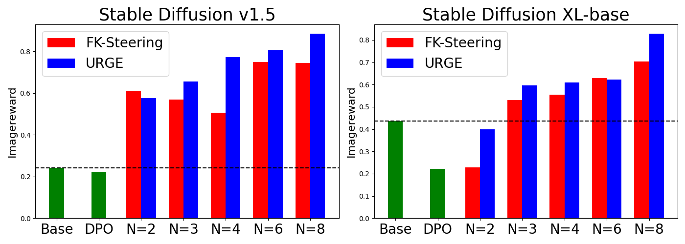
下面的粒子扩展图在 10 个提示词上比较 SD v1.5 与 SDXL,不与上表 50 个提示词的汇总数值直接对齐。在测试的 \(N=2,3,4,6,8\) 下,URGE 的 ImageReward 持续上升,多数配置高于 FK Steering;SD v1.5 的 \(N=2\) 和 SDXL 的 \(N=6\) 是例外。这是给定实验里的趋势,不是所有任务上的单调性保证。
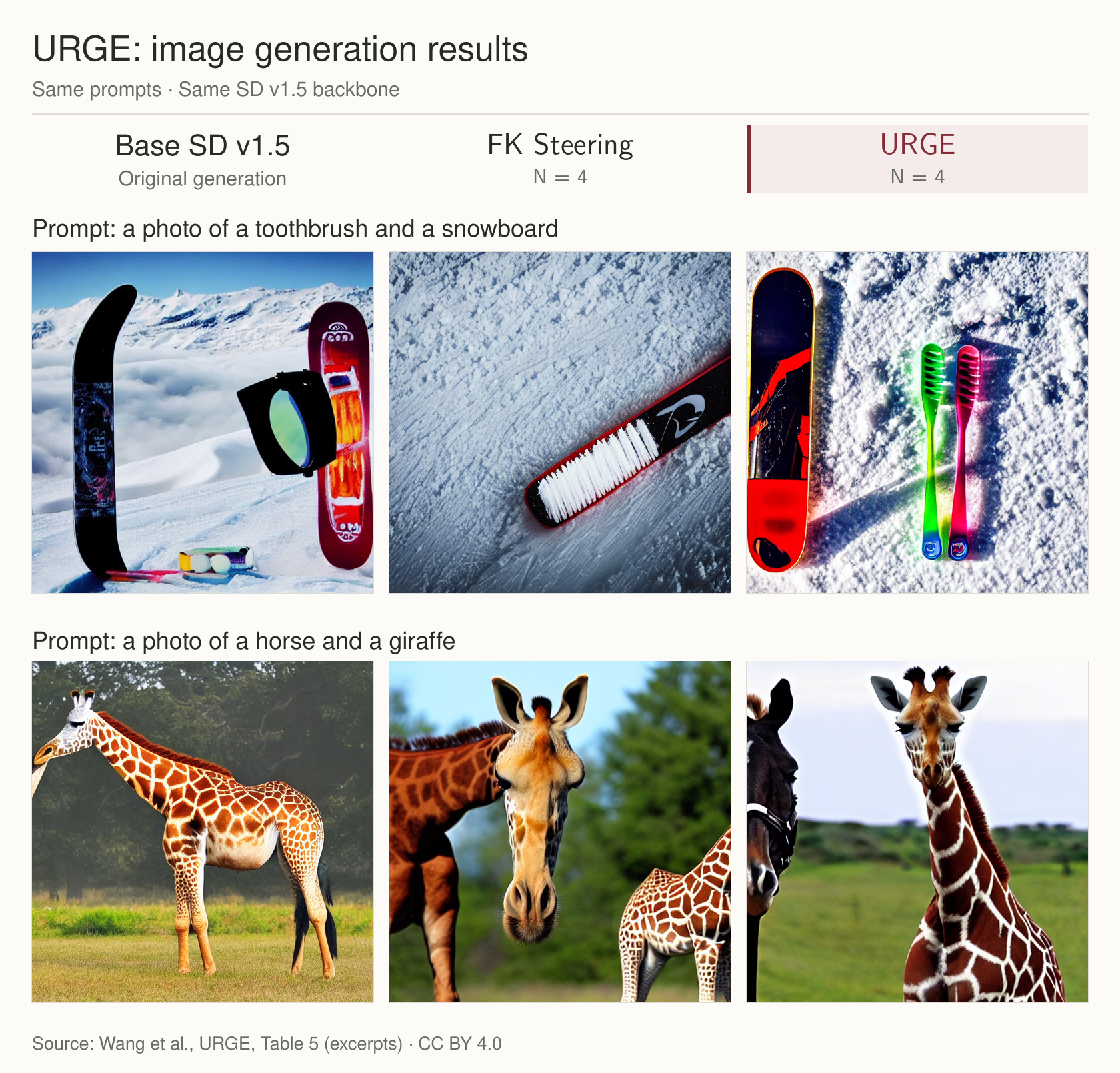
分数对应怎样的视觉变化?图 8 选出“牙刷与单板滑雪板”和“马与长颈鹿”。重点看:两个物体是否同时出现,还是被混成了一个物体?

Stein:两个中心化候选能省下多少查询?
文献 [2] 的布朗运动实验比较中心化候选与独立候选,指标 adjusted NESS 衡量归一化常数估计效率,不是图像质量。[2, §5.1]
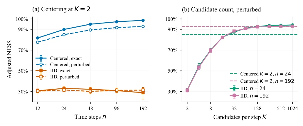
受扰动价值、\(n=192\) 时,两个中心化候选达到 92.76%,两个独立候选只有 31.40%。独立候选增至 128 和 256,才分别达到 92.38% 和 92.81%。这说明在该设置中,安排好候选之间的关系,比单纯堆数量更能稳定权重。[2, §5.1]
Stein:完整路径校正贡献了什么?
Hopper 实验固定扩散策略与 critic,检查动作的 critic 分数分布是否接近目标。三个目标分别把 30%、60%、80% 的概率放到原策略分数最高的 10% 动作中。KS 距离衡量分数累积分布的最大差距,越小越好。[2, §5.2]
| 目标强度 | 两点引导,未做外层校正 | 使用 32 条完整提议校正 |
|---|---|---|
| 30% | 0.2174 | 0.0306 |
| 60% | 0.2804 | 0.0697 |
| 80% | 0.4041 | 0.1128 |
表中是八个固定状态的平均条件 KS。指路已经有用,但完整路径校正仍大幅改善目标分布的匹配。这里测量的是固定 critic 的分数分布,不能直接解释为机器人实际回报提高了同样比例。[2, Table 2、附录 H.3]
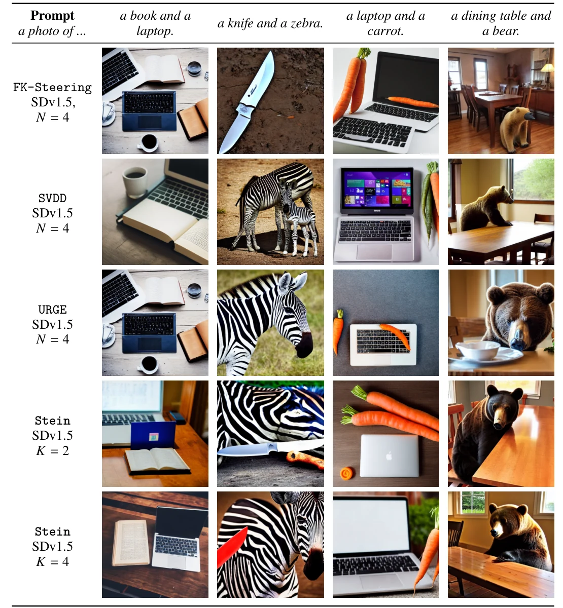
最后回到书和电脑。图 10 在同一个 SD v1.5 骨干上展示四组双物体提示词。观察它们是否同时出现、保持独立,而不是只看一张图是否漂亮。[2, §5.3]
11. 把三件事分开,算法就清楚了
引导让计算更常走向有希望的区域;独立提议避免跨路径复制带来的共同祖先;路径校正补偿不精确判断造成的概率偏差。它们解决的是三个不同问题。
URGE 说明,记录路径就能更方便地算清校正的账。Stein Guidance 再往前一步:两个对称候选提供有限差分,中心化的 \(K\) 个候选提供并行的 Stein 引导,而同一批函数值同时给出完整路径的校正权重。
不用价值导数,不等于没有方向;不复制祖先,也不等于可以不校正。把这些分工明确下来,才知道多出的计算究竟改善了什么。
12. 研究问题:怎样同时实现无导数引导与校正?
Stein Guidance 给出的一个答案,是把候选池与选择编号保留下来:候选之间的价值差提供方向,候选价值的平均与选中值提供校正因子。无导数引导与无导数校正因此来自同一个随机构造。这里“精确”指扩展空间的加权恒等式;有限次 MH 更新仍有采样误差。[2]
进一步的研究是:当候选分布不再是高斯,或者候选池随状态自适应变化时,能否仍然让同一批函数值同时支持有效引导、可验证的校正和稳定的路径权重? 检验一个新设计,除了看平均移动方向,还要证明完整权重恢复了目标分布,并控制其波动是否会随路径加深而恶化。
参考文献
[1]URGE。Chenyang Wang, Weizhong Wang, Yinuo Ren, Jose Blanchet, Yiping Lu. Simple Approximation and Derivative Free Inference Time Scaling for Diffusion Models via Sequential Monte Carlo on Path Measures. ICML 2026。正式论文页面 · arXiv · HTML 全文。
[2] Stein Guidance。Youheng Zhu, Chenyang Wang, Minshuo Chen, Yiping Lu. Stein Guidance without Gradients: Discretization Uniform Diffusion Inference Time Scaling beyond Particle SMC. 2026。PDF 全文。
Ask for “a book and a laptop,” and the model draws a laptop but forgets the book. Try again: the book appears, but the laptop disappears. If the model sometimes gets it right, can extra computation during generation make it succeed more often?
The simplest strategy is to generate several images and pick one. A more active strategy is to judge promising directions before an image is finished, then spend more computation there.
Those intermediate judgments may be wrong. And repeated selection can turn many generation paths into descendants of the same ancestor. We want to use computation effectively while keeping inaccurate judgments from distorting the final distribution.
This blog follows one thread: URGE corrects guidance using path information; independent rejection avoids shared ancestry; Stein Guidance makes both guidance and correction depend only on function values. Here, “without gradients” means without differentiating the value function. The base denoising model still runs as usual. [1] [2]
1. What should extra computation achieve?
Think of a diffusion model as a random drawing process: start from noise, denoise gradually, and finish with an image. Time runs in the generation direction here: \(0\) is the start and \(T\) is completion. The trained model defines a base distribution \(p_{\mathrm{base}}\).
Assign a score \(r(x)\) to the finished image and convert it into a positive preference weight \(\phi(x)=e^{\beta r(x)}\). Our target distribution is
\[\pi(x)=\frac{p_{\mathrm{base}}(x)\phi(x)} {\mathbb E_{p_{\mathrm{base}}}[\phi(X)]}.\]This retains the model’s original preferences while making highly rewarded outcomes relatively more likely. The parameter \(\beta\) controls the strength of that preference. [1, §2.1]
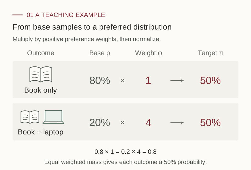
This sampling objective is related to finding the highest scoring image, but they are different objectives. Generating independent images and keeping the best generally does not sample from \(\pi\). All claims about correct sampling below refer to this specific distributional target.
There are also three distinct ways to increase computation: more denoising steps \(n\), more generation paths \(N\), or more candidates \(K\) at each step. These increase numerical depth, statistical width, and local queries, respectively. They should not all be called a “sample count.” [2, §1]
2. To choose the next step, ask about its future
A partially generated image is still blurry. Asking whether it looks like a book now may tell us little about the finished result. A better question is: if generation continues from this state, what is the average final preference weight?
\[H_t^\star(x)=\mathbb E[\phi(X_T)\mid X_t=x].\]This value function accounts for possible futures. If we knew it exactly, we could sample the next step in proportion to “base transition probability × next step’s value.” In continuous time, the corresponding guidance drift is \(\sigma\sigma^\top\nabla\log H_t^\star\), the Doob transform. [1, §1] [2, §3]
The difficulty is that \(H^\star\) itself contains a high dimensional integral. In practice, we usually have only an approximate value \(H\), for example by predicting the final image and scoring that prediction.
This separates two jobs: approximate values provide directions; correction compensates for the probability bias caused by wrong directions. Better judgments usually make correction easier, but correctness cannot rely on every judgment being accurate.
3. URGE: keep the accounts for the entire path
Guidance changes how the model moves. Many paths can reach the same endpoint, so calculating the guided endpoint density directly is difficult. URGE instead retains the actual path and computes a probability ratio for that path. [1, §2.3]
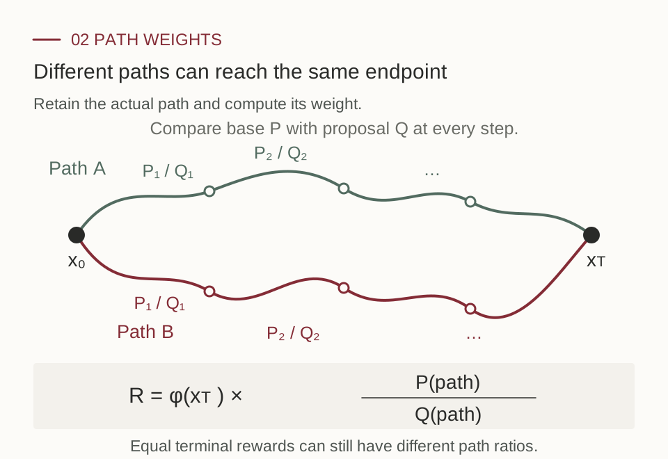
In discrete time, let \(P_k\) be the base transition density and \(Q_k\) the actual proposal density. Assume the same initial distribution and the support conditions needed for the probability ratio. For a generated path, record
\[R=\phi(X_n)\prod_{k=0}^{n-1} \frac{P_k(X_k,X_{k+1})}{Q_k(X_k,X_{k+1})}.\]Paths drawn too often under guidance should be downweighted; paths drawn too rarely should be upweighted. The terminal preference specifies what we want, and the probability ratio compensates for how we actually sample.
The continuous time counterpart is Girsanov’s change of measure. URGE computes path weights from the simulated drift and random increments, then reweights and resamples during generation. It is itself an SMC method; the expandable explanation below connects its path weights to particle weights. [1, §2.3]
URGE and particle SMC: condition on the endpoint, save derivatives, retain more variance
Keep a separate account for each path, or first combine accounts that reach the same endpoint? Both methods propagate, weight, and resample. URGE’s weight depends on the realized path. The particle perspective averages over paths with the same endpoint using their conditional probabilities, keeping a weight that depends only on the current state. The particle correctors discussed here are specifically FK Corrector and AFDPS.
Under the same proposal law \(Q\), let \(W\) be the weight of a path segment. Averaging over the unobserved path while fixing its endpoint gives
\[\overline W(x)=\mathbb E_Q[W\mid X_t=x].\]Intuitively, an endpoint statistic need not distinguish a detour from a direct route if both arrive at the same \(x\). For any suitable endpoint function \(f\), the tower property gives
\[\mathbb E_Q[Wf(X_t)] =\mathbb E_Q[\overline W(X_t)f(X_t)].\]Thus, weighting paths and then retaining only endpoints gives the same weighted marginal distribution as first averaging path weights conditional on the endpoint and then weighting endpoints. The normalizing constants also agree, by taking \(f=1\).
For URGE’s short path increments, the paper further shows, under the relevant regularity and marginal matching conditions,
\[\lim_{h\downarrow0} \frac{\mathbb E_Q[W_{t-h,t}\mid X_t=x]-1}{h} =\lambda_{\mathrm{particle}}(x,t),\]where the right side is the FK Corrector / AFDPS particle correction potential. The conditional averaging identity is exact over a finite interval; identifying the paper’s particle correction potential requires the short time limit. This does not mean that two finite particle implementations select identical particles at every resampling step. [1, Theorem 3.3]
The benefit: Itô’s formula rewrites derivative terms as increments recorded along a simulated path. Let \(\ell_t\) be the log intermediate preference weight, with \(\ell_T=\log\phi\), and write the guided proposal as \(dX=(b+\sigma u)\,dt+\sigma\,dB^Q\). URGE’s incremental weight is
\[\log W_{s,t} =\ell_t(X_t)-\ell_s(X_s) -\int_s^t u_\tau^\top dB_\tau^Q -\frac12\int_s^t\|u_\tau\|^2d\tau.\]This uses endpoint function values, the actual change in drift, and noise already generated by the simulation. Why can it replace an expression involving derivatives? Itô’s formula writes the same function increment as
\[d\ell_t(X_t) =\left[\partial_t\ell_t+(b+\sigma u)\cdot\nabla\ell_t +\tfrac12\operatorname{tr}(\sigma\sigma^\top\nabla^2\ell_t)\right]dt +(\sigma^\top\nabla\ell_t)^\top dB_t^Q.\]The right side contains time derivatives, gradients, and a Hessian. Along a simulated path, the left side integrates to a difference of function values. Together with the Girsanov path ratio, this avoids additional derivative or marginal score evaluations for correction. If guidance itself uses \(u=\sigma^\top\nabla G\), that guidance gradient is still needed.
The cost: even with the same endpoint, different realized paths can produce different weights. For square integrable \(W\), the law of total variance gives
\[\operatorname{Var}_Q(W) =\operatorname{Var}_Q(\overline W(X_t)) +\mathbb E_Q[\operatorname{Var}_Q(W\mid X_t)] \ge\operatorname{Var}_Q(\overline W(X_t)).\]Conditional averaging is a Rao–Blackwellization: it removes weight noise caused by different paths reaching the same endpoint. URGE uses the realized path weight, saving the cost of conditional averaging or explicit derivative evaluations while retaining this extra variance. The inequality is strict whenever weights genuinely vary conditional on the endpoint.
The Itô rewrite is an identity and does not itself increase variance. The extra variance is the cost of retaining path randomness relative to the exact conditional average. This comparison concerns raw weights under the same proposal. Final algorithmic error also depends on discretization, derivative estimation, resampling, and computational budget.
4. Many paths may already belong to one family
SMC repeatedly copies particles with large weights and removes those with small weights. A copy inherits the particle’s current state and the history that produced it. The number of particles still on screen and the amount of independent early exploration they retain are different quantities.
Imagine four people solving a problem. Every so often, each chooses a draft according to its score and continues from it. After several rounds, four answers may remain on the table, yet all descend from one early draft. Later work can differ while still inheriting the same crucial early choice.
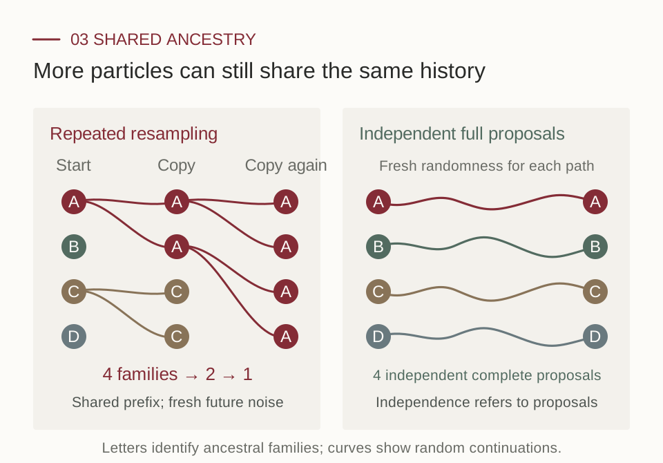
Follow the left panel: the first round retains descendants of A and C, losing the early exploration of B and D. The second retains only family A. The four particles can occupy different positions while still depending on the same early random history. On the right, four complete generations each use their own random numbers, preserving four independent opportunities to explore.
A simple model shows why this matters for statistical precision. Write the final outcomes as \(X_T^{(i)}=A+\varepsilon_i\): \(A\) is the inherited random prefix, while the later noises \(\varepsilon_i\) are independent, identically distributed, and independent of \(A\). Averaging \(N\) descendants gives
\[\operatorname{Var}\!\left(\frac1N\sum_{i=1}^N X_T^{(i)}\right) =\operatorname{Var}(A)+\frac{\operatorname{Var}(\varepsilon_1)}N.\]Averaging reduces independent noise from the later stages, but it does not average away the early error inherited by everyone. This additive model illustrates correlation; it is not a representation of every diffusion process.
ESS measures only how uniform the current weights are. Resampling usually resets them to equal values, so \(\mathrm{ESS}=N\) can hold even when all four particles belong to family A. ESS does not track the family tree and cannot establish independence. Increasing denoising depth can create more opportunities for ancestral merging if it also increases the number of resampling rounds. [2, §1, Appendix E]
A rigorous example: resampling at every step can accumulate error with depth
Reference [2] constructs a Brownian example with a fixed terminal target and local Bellman error \(O(1/n)\). With full multinomial resampling at every numerical step, the distribution of one final particle satisfies
\[\left\|\nu_{n,N}^{\mathrm{SMC}}-\pi\right\|_{\mathrm{TV}} \asymp\frac nN,\qquad 2\le n\le N.\]Total variation measures the largest difference between the probabilities that two distributions assign to the same event. This result concerns the constructed model and full resampling at every step. It is not a lower bound for every SMC method, and does not rule out the value of sparse or adaptive resampling. [2, Theorem 1]
5. Why correct paths that never copy each other?
Reject this step, keep your own draft
A natural alternative is sequential rejection sampling: propose a move from the current state, then accept or reject according to the candidate’s value. On rejection, retain your own prefix and retry only this step, instead of copying another path’s history.
Given a known valid bound \(0<H_{k+1}(y)\le M_k(x)\), draw \(Y\) from the base transition \(P_k(x,\cdot)\) and accept with probability \(H_{k+1}(Y)/M_k(x)\). Repeat until accepted, then advance. Independent repetitions of this complete procedure have no shared ancestry across paths. This is the mechanism on the right below.
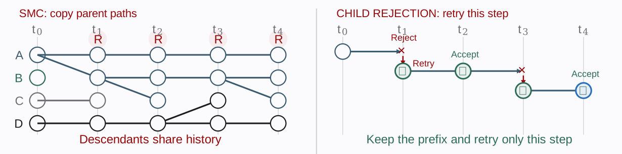
This also differs from the outer MH correction introduced later. Here, rejection concerns one substep; outer MH accepts or retains an entire path.
Independent paths can still follow inaccurate directions
One advantage of SMC is that it keeps a running account of weights. For a fixed initial state and terminal value \(H_n=\phi\), use incremental weights \(H_{k+1}(X_{k+1})/H_k(X_k)\) under the base transitions. Then
\[\frac{H_1(X_1)}{H_0(X_0)} \frac{H_2(X_2)}{H_1(X_1)}\cdots \frac{\phi(X_n)}{H_{n-1}(X_{n-1})} =\frac{\phi(X_n)}{H_0(X_0)}.\]Intermediate judgments are provisional entries: add one now, subtract it next time. They need not equal the true future value for the correct unnormalized target to depend only on the terminal preference. This is an identity for the weights, not a claim that finite particle SMC is exact. [2, Appendix E.2]
Local rejection alone behaves differently. Each step normalizes candidate values into probabilities. Its denominator is the true average next value from the current state, which need not equal the current approximate prediction. Adjacent value terms can still cancel, but the ratios left by disagreement between prediction and actual average usually do not. [2, §3, equations (10)–(11)]
A two step teaching example makes this clear. The base model chooses routes A and B with equal probability. Each route then reaches its own distinct endpoint, and both terminal preferences equal 1, so the target should assign each route half the mass. But an intermediate predictor gives A a value of 9 and B a value of 1:
| Disjoint routes | Target probability | Intermediate prediction | Probability after local rejection |
|---|---|---|---|
| A | 50% | 9 | 90% |
| B | 50% | 1 | 10% |
At the endpoint, both rewards are correct but equal to 1, so the last step does not distinguish the routes. The extra chances given to A earlier are not automatically refunded by accurate terminal scores.
Correction multiplies A’s relative weight by \(1/9\) and B’s by \(1\). Both weighted masses become \(0.1\), giving \(50\%\) each after normalization. Alternatively, accept A at the end with probability \(1/9\) and always accept B. This restores the probabilities without copying another path’s prefix. These numbers illustrate the mechanism; they are not experimental results.
The formula: why locally exact sampling can remain globally biased
Write
\[G_k(x)=(P_kH_{k+1})(x),\qquad Q_k^H(x,dy)=\frac{P_k(x,dy)H_{k+1}(y)}{G_k(x)}.\]With a valid envelope, local rejection samples exactly from \(Q_k^H\). Relative to the final target \(\Pi_n\propto\phi(X_n)P_n\), however, the complete path still has weight
\[R_H=\phi(X_n)\frac{dP_n}{dQ^H}(X_{0:n}) =H_0(x_0)\prod_{k=0}^{n-1}\frac{G_k(X_k)}{H_k(X_k)}.\]Exact Doob values satisfy \(G_k=H_k\), making the weight constant, so local sampling suffices. Approximate values generally leave a product that depends on the path. If that product happens to be constant, correction is also unnecessary; otherwise it is the missing complete path correction. [2, §3, Appendix C.3]
In the two step example, \(G_0=5\) and \(G_1(A)=G_1(B)=1\). The exact path weights are therefore \(5/9\) and \(5\). Removing their shared factor of 5 gives the relative weights \(1/9\) and \(1\) used above.
The difficulty is that \(G_k\) is itself an integral and is usually unavailable exactly. A finite candidate pool must provide computable correction information as well as a next step. For a random initial state, the initial distribution factor must also be included; the constant factor argument for a fixed start cannot simply be reused. [2, Proposition 22]
Another cost of explicit guidance: why can correction need second derivatives?
Start with steering. Changing the drift to \(b+a\nabla\log H\), where \(a=\sigma\sigma^\top\), asks which direction increases the value at the current point. That requires a first derivative. But \(H\) is approximate. After generating a complete path, we still need to ask: how much did these intermediate judgments distort its sampling probability, and what weight should determine whether we keep it?
The discrete correction above already gives a clue: each step leaves a factor \(G_k/H_k\), with \(G_k=P_kH_{k+1}\). The numerator is the actual average next value after a step of the base dynamics; the denominator is the current prediction of the future. Exact values make them agree. Their discrepancy for approximate values is the Bellman defect that must be accumulated along the path.
Why does computing this average involve a second derivative? A random step can move left or right. The first order changes cancel on averaging, but curvature that bends both sides up or down remains. Temporarily ignoring time and drift, the one dimensional Taylor expansion is
\[H(x+\sqrt h Z) =H(x)+\sqrt h\,H'(x)Z+\frac h2 H''(x)Z^2+\cdots, \qquad Z\sim N(0,1).\]Since \(\mathbb EZ=0\) and \(\mathbb EZ^2=1\), under suitable smoothness and integrability,
\[\mathbb E[H(x+\sqrt h Z)]-H(x) =\frac h2 H''(x)+o(h).\]For example, take \(H_+(x)=e^{cx^2}\) and \(H_-(x)=e^{-cx^2}\) with \(c>0\). At \(x=0\), both have value 1 and gradient 0, giving the same instantaneous guidance. Yet one is a valley and the other a hilltop. After a small random step, their average values become \(1+ch+O(h^2)\) and \(1-ch+O(h^2)\), respectively. Identical values and gradients can require opposite local probability corrections. Curvature supplies the missing information.
Restoring time evolution, base drift, and multidimensional noise gives the relative defect per unit time:
\[\mathcal E_t(x) =\frac{\partial_tH_t+b_t\cdot\nabla H_t +\tfrac12\operatorname{tr}(a_t\nabla^2H_t)}{H_t}(x).\]The three terms describe changes due to time, base drift, and the interaction of noise with curvature. The last contracts the Hessian with the noise covariance. Computing it need not require storing the full Hessian, but it still requires second spatial derivative information.
How does this enter the final accept or reject decision? For a fixed initial state, \(H_T=\phi\), positive and sufficiently smooth \(H\), and a valid change of measure, the continuous time proposal with drift \(b+a\nabla\log H\) has unnormalized complete path correction weight
\[R_H=H_0(x_0)\exp\!\left(\int_0^T\mathcal E_t(X_t)\,dt\right).\]The terminal preference is already included through \(H_T=\phi\). The exponential accumulates probability corrections along the whole path and enters the MH ratio of new and old path weights. A valid weight bound also permits complete path rejection sampling. The acceptance formula is simple; computing its path weight is the challenge. Along the residual route, the gradient provides guidance, while time and second spatial derivatives enter correction. In discrete time, the counterpart is the accumulated \(\log(G_k/H_k)\) above. [2, §4, equation (11)]
How can URGE avoid explicit Hessians?
The expression above rewrites a path probability ratio as a value function residual. URGE retains the actual drift and noise increments and computes correction directly through the Girsanov path ratio, avoiding explicit time derivatives and Hessians. If its drift uses \(\nabla\log H\), constructing the proposal still requires value gradients. Higher derivatives are a cost of evaluating the residual directly, not an unavoidable cost of every correction method. [1, §2.2–2.4]
A continuous time identity also does not make an arbitrary discretization exact. An implementation needs correction weights matched to its actual discrete proposal.
We therefore need two mechanisms designed together: use function values to steer toward promising regions, while keeping a probability account that can also be computed from function values. The next section starts with two symmetric candidates and shows how the same queries can serve both purposes.
6. Why do two symmetric candidates produce a log gradient?
The symmetric difference supplies a directional derivative of value. Normalizing the selection probabilities divides it by the current value, giving \(\nabla H/H=\nabla\log H\).
Write the position after the base drift as \(\mu=x+hb(x)\). Draw a Gaussian perturbation \(\delta=\sqrt h\,\sigma Z\) with \(Z\sim N(0,I)\), then construct two symmetric candidates and query their values:
\[Y^\pm=\mu\pm\delta,\qquad H^\pm=H(Y^\pm).\]Select one candidate with probability \(p_\pm=H^\pm/(H^++H^-)\). Conditional on the current state and perturbation, the mean displacement is exactly
\[\mathbb E[Y^J-\mu\mid x,Z] =\delta\frac{H^+-H^-}{H^++H^-}.\]Expand the two values to first order: their difference cancels the constant term and leaves \(2\delta^\top\nabla H(\mu)\), while their sum has leading term \(2H(\mu)\). For a small perturbation,
\[\frac{H^+-H^-}{H^++H^-} \approx\frac{\delta^\top\nabla H(\mu)}{H(\mu)} =\delta^\top\nabla\log H(\mu).\]Substituting into the mean displacement gives the leading term \(\delta\delta^\top\nabla\log H(\mu)\). Average over the random direction and use \(\mathbb E[\delta\delta^\top\mid x]=h\sigma\sigma^\top\) to obtain
\[\mathbb E[Y^J\mid x] =\mu+h\sigma\sigma^\top\nabla\log H(\mu)+o(h).\]This is log gradient guidance scaled by the noise covariance. Implementation only queries two function values and selects one candidate proportionally; the gradient appears in the analysis of the mean displacement and need not be computed. The small step limit requires smooth positive \(H\) and integrable remainder terms. It describes the leading mean drift; the finite step transition law still requires correction. [2, §3.1.1, equation (5), Appendix B.2.1]
7. Stein’s identity: from two points to K parallel candidates
Two points reveal directional information. Can we query \(K\) directions simultaneously using only function values? Gaussian Stein’s identity provides the connection:
\[\mathbb E[Zf(Z)]=\mathbb E[\nabla f(Z)],\qquad Z\sim N(0,I).\]The left side uses values; the right side is an average gradient. Intuitively, the average of “random direction × value” points toward directions that tend to receive higher values. For \(Y=\mu+\sqrt h\,\sigma Z\),
\[\mathbb E[ZH(Y)]=\sqrt h\,\sigma^\top\mathbb E[\nabla H(Y)].\]This holds under the appropriate Gaussian integration by parts conditions. [2, §3.1.2, Proposition 6]
Preserve symmetry by making the directions sum to zero
The two candidate method has \(Z_1+Z_2=0\). For \(K\ge2\), draw independent standard Gaussians \(G_i\), subtract their average, and restore each direction’s variance:
\[\bar G=\frac1K\sum_iG_i,\qquad Z_i=\sqrt{\frac K{K-1}}(G_i-\bar G),\qquad \sum_iZ_i=0.\]Each \(Z_i\) remains marginally standard Gaussian, while directions in the pool are dependent. Construct candidates, query all values in parallel, then randomly select one in proportion to its value:
\[Y_i=\mu+\sqrt h\,\sigma Z_i,\qquad H_i=H(Y_i),\qquad \Pr(J=i\mid Y_{1:K})=\frac{H_i}{\sum_jH_j}.\]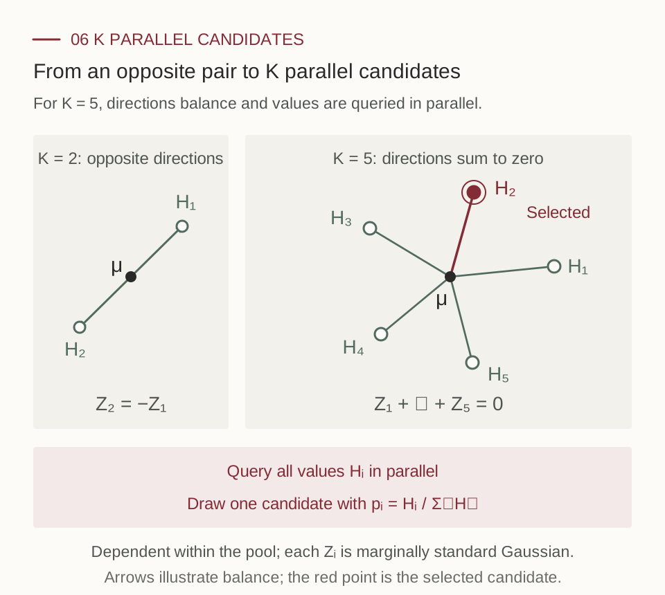
Given a candidate pool \(U\), the mean displacement is exactly
\[\mathbb E[Y_J-\mu\mid U] =\sqrt h\,\sigma\frac{\sum_iZ_iH_i}{\sum_iH_i}.\]Finite queries replace the expectations in ideal value tilting. For \(K=2\), \(Z_1=(G_1-G_2)/\sqrt2=-Z_2\), recovering the finite difference construction. Odd values of \(K\) work too; candidates need not be arranged in pairs. [2, equations (7)–(8)]
Why does centering improve the variance by one order in h?
Candidate perturbations have size \(\sqrt h\). Centering cancels the first order random term in the Taylor expansion exactly, leaving second order fluctuations of size \(h\). Squaring their size changes the variance from order \(h\) to order \(h^2\). Here is the calculation. [2, Remark 2]
Fix the current state, so \(\mu,\sigma\) are known. We study fluctuations of the average candidate value \(S=K^{-1}\sum_iH(\mu+\sqrt h\,\sigma Z_i)\). Write its true mean as \(G_h=\mathbb ES\), and abbreviate
\[g=\sigma^\top\nabla H(\mu),\qquad A=\sigma^\top\nabla^2H(\mu)\sigma,\qquad \bar Z=\frac1K\sum_iZ_i.\]Expand each candidate value to second order, average, and subtract the expectation:
\[\begin{aligned} S-G_h &=\sqrt h\,g^\top\bar Z\\ &\quad+\frac h{2K}\sum_{i=1}^K \left(Z_i^\top AZ_i-\operatorname{tr}A\right)+r_h. \end{aligned}\]The first line is first order noise from the gradient; the second is second order noise from curvature. The following asymptotic formulas hold for fixed \(K\) as \(h\to0\). If \(H\) is twice continuously differentiable with bounded Hessian, the remainder \(r_h\) has root mean square size \(o(h)\).
Independent candidates: the first order term vanishes only in expectation. When the \(Z_i\) are independent, \(\mathbb E\bar Z=0\), but each realized \(\bar Z\) is still random, with \(\operatorname{Cov}(\bar Z)=I/K\). The first order term therefore usually determines the leading variance:
\[\operatorname{Var}(S_{\mathrm{iid}}) =\frac{h\|g\|^2+o(h)}{K}.\]Centered candidates: the first order term vanishes in every draw. The construction above guarantees \(\sum_iZ_i=0\), so the entire term \(\sqrt h\,g^\top\bar Z\) disappears. The leading remaining random term has coefficient \(h\) rather than \(\sqrt h\). Calculating the variance of this quadratic term gives
\[\operatorname{Var}(S_{\mathrm{centered}}) =\frac{h^2}{2(K-1)}\|A\|_F^2+o(h^2).\]Here \(\|A\|_F^2\) is the sum of squared matrix entries. The extra order in \(h\) comes from reducing the fluctuation size from \(\sqrt h\) to \(h\) and then squaring it. It does not require more candidates.
Each centered direction remains marginally standard Gaussian, so both constructions satisfy \(\mathbb ES=G_h\) and estimate the same normalizing constant. If \(G_h\) has a uniform positive lower bound, division by \(G_h^2\) preserves these variance orders: the variance of the normalized average \(S/G_h\) improves from \(O(h/K)\) to \(O(h^2/(K-1))\). This concerns random error; the smoothing difference between \(G_h\) and \(H(\mu)\) can still be \(O(h)\). If \(g=0\), the independent construction’s first order term already vanishes.
Calculate the coefficient: why is the denominator K−1?
The centered directions are correlated:
\[\operatorname{Cov}(Z_i,Z_j)=-\frac{I}{K-1}, \qquad i\ne j.\]Write \(q_i=Z_i^\top AZ_i\). The Gaussian fourth moment formula gives
\[\operatorname{Var}(q_i)=2\|A\|_F^2,\qquad \operatorname{Cov}(q_i,q_j) =\frac{2\|A\|_F^2}{(K-1)^2}\quad(i\ne j).\]Include both the diagonal and cross terms when computing the variance of the average:
\[\begin{aligned} \operatorname{Var}\!\left(\frac1K\sum_iq_i\right) &=\frac{2\|A\|_F^2}{K^2} \left(K+\frac{K(K-1)}{(K-1)^2}\right)\\ &=\frac{2\|A\|_F^2}{K-1}. \end{aligned}\]Multiplying by the squared Taylor coefficient \(h^2/4\) gives \(h^2\|A\|_F^2/[2(K-1)]\). Negative correlation between directions cancels the linear noise, but the quadratic terms have positive covariance, so the calculation must use their actual joint distribution. [2, Appendix B.3]
There is also a bound beyond the leading asymptotic term. Let \(F(z)=H(\mu+\sqrt h\,\sigma z)\). If \(F\) and its derivatives through order two are square integrable under the standard Gaussian law, and \(G_h>0\), [2, Theorem 8] gives, for every \(K\ge2\),
\[\operatorname{Var}\!\left(\frac S{G_h}\right) \le \frac{h^2}{2(K-1)G_h^2} \mathbb E\left\| \sigma^\top\nabla^2H(\mu+\sqrt h\,\sigma Z)\sigma \right\|_F^2.\]A uniform bound on this relative curvature term yields the uniform \(O(h^2/(K-1))\) guarantee. The Hessian appears only in the error analysis. Constructing candidates, computing \(S\), and correcting the path still use only function values.
Why can guidance remain biased when the value estimators are unbiased?
Let \(G=\mathbb E[H(Y)]\). Stein’s identity gives
\[\widehat v=\frac1{K\sqrt h}\sum_iZ_iH(Y_i),\qquad \mathbb E\widehat v=\sigma^\top\mathbb E\nabla H(Y),\qquad \mathbb ES=G.\]But generally \(\mathbb E[\widehat v/S]\ne\mathbb E[\widehat v]/\mathbb E[S]\). Unbiased numerator and denominator estimators do not make their ratio unbiased. Bias from finite candidate pools and imperfect values still requires the path weights in the next section. [2, Proposition 6, Theorem 11]
8. Correct the entire path after generation
Section 5 left an obstacle: the ideal local normalizer \(G_k=P_kH_{k+1}\) is difficult to compute. A finite candidate pool provides a way forward: retain the average of the same value queries to construct an exact augmented space weight, without evaluating the integral exactly. [2, §3.2, Theorem 12]
\[R=\phi(X_n)\prod_{k=0}^{n-1} \frac{S_k}{H_{k+1}(X_{k+1})},\qquad S_k=\frac1K\sum_{i=1}^K H_{k+1}(Y_{k,i}).\]This weight addresses the bias left by both approximate values and finite candidate selection, using no extra value queries or derivatives. Its validity comes from an augmented space containing the candidate pools and selection indices. Arbitrarily replacing \(G_k\) with an unbiased estimator would not automatically be valid.
Now apply independence Metropolis–Hastings to entire paths. If new and old path weights are \(R_{\mathrm{new}}\) and \(R_{\mathrm{old}}\), accept with probability
\[\alpha=\min\{1,R_{\mathrm{new}}/R_{\mathrm{old}}\}.\]On acceptance, move to the new path. On rejection, retain the old path and its old weight. Compare the corrected path weights, not just the terminal rewards. [2, Algorithm 2]
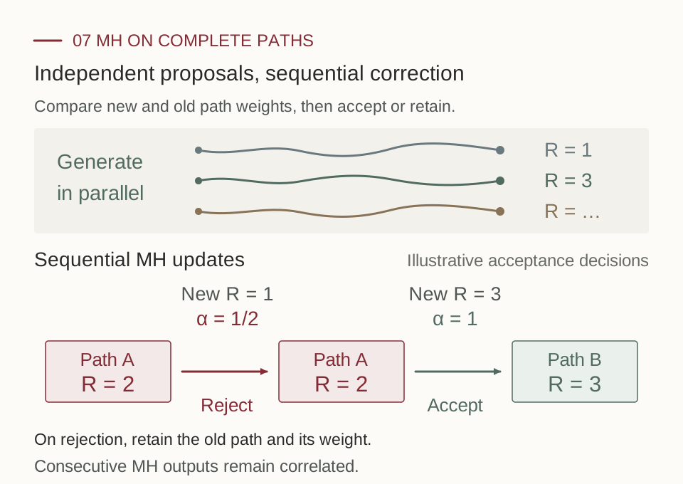
Proposal paths are independent; consecutive outputs from one MH chain remain correlated. A finite number of updates also leaves initialization error. Independent outputs require independent repetitions of the full procedure. With a known valid bound on the complete path weight, rejection of entire paths can instead give independent exact samples from the finite grid target. Here we focus on outer MH with a fixed computation budget. [2, Algorithm 2, Appendix G.2]
Why the weight works: one exact cancellation
Given the candidate pool, \(S=K^{-1}\sum_iH(Y_i)\) and candidate i is selected with probability \(H(Y_i)/(KS)\). Hence
\[\mathbb E\!\left[\frac S{H(Y_J)}f(Y_J)\mid U\right] =\sum_i\frac{H(Y_i)}{KS}\frac S{H(Y_i)}f(Y_i) =\frac1K\sum_i f(Y_i).\]Average over the pool. Each candidate has the correct base transition marginal, so the right side recovers the base transition. Repeating over time and multiplying by \(\phi(X_n)\) gives
\[\mathbb E_{\widetilde Q}[RF(X_{0:n})] =\mathbb E_{P_n}[\phi(X_n)F(X_{0:n})].\]This restores the weighted path target, beyond merely correcting an average drift. That target is invariant for the resulting MH chain; approaching it in finite time still requires convergence analysis. [2, Theorem 12]
9. Can more denoising steps stop forcing us to add more paths?
Fix total time \(T\) and set \(h=T/n\). The centered pool’s per step normalization variance is \(O(h^2/(K-1))\). Across \(n\) steps, the corresponding scale is
\[\frac{nh^2}{K-1}=\frac{Th}{K-1}.\]This pool noise contribution decreases as the grid becomes finer. The approximate value’s Bellman error is a separate term; a larger candidate pool does not automatically remove it. [2, §4]
With a fixed initial state, \(H_n=\phi\), uniform positive upper and lower value bounds, and bounded second spatial derivatives and noise coefficients, the paper proves that the number of complete proposals required for prescribed finite grid sampling accuracy need not grow with denoising depth. Constants may depend on dimension and value bounds; the claim is not dimension independence. [2, Theorem 4]
Depth is still not free. There are \(m+1\) complete proposals for \(m\) outer updates plus initialization, and the value query count is \(Kn(m+1)\). The result addresses whether longer paths force us to increase the number of paths as well. It does not eliminate the cost of making each path longer.
With a fixed query budget per path, are two candidates already enough?
Fix a proposal budget \(B=Kn\). Then
\[\frac{Th}{K-1}=\frac{T^2}{B}\frac K{K-1}.\]For \(K\ge2\), the last factor lies between 1 and 2. Considering only pool noise, two candidates already achieve the same budget order. More candidates increase parallelism but reduce the number of steps available within the same budget, so they do not necessarily reduce total error. [2, §4]
These statements concern the discrete model’s target distribution. Its numerical error relative to the continuous time diffusion target needs separate analysis. Numerical error, value approximation error, and finite computation sampling error should be accounted for separately.
10. Experiments: URGE, then Stein
URGE: first test a distribution with a known answer
URGE uses a Gaussian mixture in 30 dimensions with 40 components. After applying a quadratic reward, the target remains analytically available, so distributional accuracy can be checked directly. The following excerpt from Table 2 compares methods using both guidance \(G=r\) and resampling. [1, §4.1, Table 2]
| Method | MMD ↓ | SWD ↓ | Mean error ↓ | Covariance error ↓ |
|---|---|---|---|---|
| FK Steering | 0.07 | 0.85 | 4.86 | 198.20 |
| URGE | 0.06 | 0.62 | 3.20 | 181.31 |
Lower is better for all four metrics. MMD and SWD measure distributional differences; mean and covariance errors describe the center and spread of the point cloud. In this experiment, URGE is closer to the target: SWD decreases from 0.85 to 0.62, and mean error from 4.86 to 3.20. This supports the effectiveness of correction, but a smaller empirical error does not establish exact sampling.
How was this experiment run?
It uses 8192 particles and 500 discretization steps, with resampling when ESS falls below 80% of the particle count. URGE’s original table averages five random seeds. SWD can be understood by projecting a high dimensional point cloud in many directions and comparing the resulting one dimensional distributions. [1, Table 2, Appendix C]
URGE: what changes at the same particle count?
The image generation evaluation uses 50 prompts with three random seeds each. Below are three methods from Table 4, all using four particles. Higher is better for every metric. [1, §4.3, Table 4]
| Method, all with 4 particles | CLIP ↑ | HPS ↑ | ImageReward ↑ | GenEval ↑ |
|---|---|---|---|---|
| FK Steering | 0.2901 | 0.2849 | 0.8397 | 0.7200 |
| FK Steering with gradient guidance | 0.2899 | 0.2839 | 0.7906 | 0.7467 |
| URGE | 0.2997 | 0.2927 | 0.9955 | 0.7800 |
CLIP measures semantic agreement between image and text. HPS and ImageReward are learned preference scores. GenEval checks requested conditions such as the presence of objects. Relative to FK Steering, URGE increases ImageReward from 0.8397 to 0.9955 and GenEval from 0.7200 to 0.7800. Equal particle counts do not imply equal measured runtime.
Sampling settings and the scope of the comparison
This evaluation uses 100 DDIM steps, noise parameter 1, CFG scale 7.5, and resampling every 20 steps. [1, Appendix C]
The scaling figure below compares SD v1.5 and SDXL on 10 prompts, so it should not be equated directly with the 50 prompt aggregate above. Across the tested \(N=2,3,4,6,8\), URGE’s ImageReward increases and exceeds FK Steering in most configurations. Exceptions are \(N=2\) for SD v1.5 and \(N=6\) for SDXL. This is an observed trend in the experiment, not a universal monotonicity guarantee.
What visual changes do these scores represent? Figure 8 selects “a toothbrush and a snowboard” and “a horse and a giraffe.” Look for whether both objects appear separately or become fused into one object.
Stein: how many queries can two centered candidates save?
The Brownian experiment in [2] compares centered and independent candidates. Its adjusted NESS metric measures the efficiency of normalizing constant estimation, not image quality. [2, §5.1]
With perturbed values and \(n=192\), two centered candidates reach 92.76%, compared with 31.40% for two independent candidates. Independent pools need 128 and 256 candidates to reach 92.38% and 92.81%, respectively. In this setting, arranging dependence within the pool stabilizes weights more effectively than simply adding candidates. [2, §5.1]
Stein: what does complete path correction contribute?
The Hopper experiment fixes the diffusion policy and critic, then tests whether the critic score distribution of generated actions matches the target. Three targets place 30%, 60%, or 80% of the mass on the top 10% of actions ranked by the original policy’s critic scores. KS distance measures the largest difference between score cumulative distributions; smaller is better. [2, §5.2]
| Target strength | Two candidate guidance without outer correction | Correction with 32 complete proposals |
|---|---|---|
| 30% | 0.2174 | 0.0306 |
| 60% | 0.2804 | 0.0697 |
| 80% | 0.4041 | 0.1128 |
These are mean conditional KS distances across eight fixed states. Guidance helps, but complete path correction still substantially improves agreement with the target. The metric concerns a fixed critic’s score distribution; it cannot be interpreted as the same proportional improvement in actual robot returns. [2, Table 2, Appendix H.3]
Finally, return to the book and laptop. Figure 10 shows four prompts, each with two objects, using the same SD v1.5 backbone. Check whether both objects appear and remain distinct, rather than judging only visual appeal. [2, §5.3]
11. Keep the three jobs separate
Guidance sends computation toward promising regions. Independent proposals avoid shared ancestry caused by copying across paths. Path correction compensates for probability bias from inaccurate judgments. They solve three different problems.
URGE shows how retaining paths makes correction easier to compute. Stein Guidance takes another step: two symmetric candidates provide a finite difference, centered pools of \(K\) candidates provide parallel Stein guidance, and the same function values provide complete path correction weights.
Function values can reveal a direction without value derivatives. Avoiding shared ancestry still leaves a need for correction. Keeping these roles clear tells us what extra computation actually improves.
12. Research question: guidance and correction without derivatives
Stein Guidance offers one answer by retaining the candidate pool and the selected index: differences between candidate values provide direction, while the pool average and the selected value provide the correction factor. Both operations arise from the same random construction. Here, “exact” refers to the weighting identity on the augmented space; a finite number of MH updates still leaves sampling error. [2]
A further research question is: if candidate distributions are no longer Gaussian, or candidate pools adapt to the current state, can the same function queries still provide effective guidance, verifiable correction, and stable path weights? A new design must establish more than a useful mean direction: its complete weight must recover the target distribution, and its fluctuations must be controlled as paths become deeper.
References
[1] URGE. Chenyang Wang, Weizhong Wang, Yinuo Ren, Jose Blanchet, Yiping Lu. Simple Approximation and Derivative Free Inference Time Scaling for Diffusion Models via Sequential Monte Carlo on Path Measures. ICML 2026. Proceedings · arXiv · Full text in HTML.
[2] Stein Guidance. Youheng Zhu, Chenyang Wang, Minshuo Chen, Yiping Lu. Stein Guidance without Gradients: Discretization Uniform Diffusion Inference Time Scaling beyond Particle SMC. 2026. Full paper (PDF).